Before I make a post on Parks-McClellan filter design, I want to talk about a paper I found awhile back when I was looking around on the internet for existence of a 2-dimensional or N-dimensional filter design equivalent to Parks-McClellan. I found a paper called Equiripple FIR Filter Design by FFT Algorithm (microsoft academic link , too lazy to find the paper), and it promises Parks-McClellan like filter results but using a much simpler method that simply relies on FFTs. This is the first time I read a not-already-proven research paper (say, the original OFDM paper or the “Gap” paper by Forney), and it was too good to be true. In fact, it actually sucks, and it’s easily apparent if you think about the process, but the paper make it sound so legit. I couldn’t even recreate the results with both my code and an implementation from their university that I found, so this is complete bullshit.
The algorithm can be summarized as follows:
0. Decide on a ripple  , a large N number of frequency points, and an L<N length of an FIR filter you'd like, L being an odd number so we can have a linear phase or zero phase FIR filter.
1. initialize your ideal filter, ![B[k]](https://s0.wp.com/latex.php?latex=B%5Bk%5D&bg=eeeeee&fg=666666&s=0&c=20201002) using a large number of discrete frequency points, say N points. Of course, for a low pass filter, that simply means make a rect function around the 0 index.
using a large number of discrete frequency points, say N points. Of course, for a low pass filter, that simply means make a rect function around the 0 index.
2. IFFT your filter, and window it to the number of samples you want your zero-phase FIR filter to be. Say, if you want a filter of L samples such that L is odd, then we want samples N-floor(L/2):N-1 and 0:floor(L/2), basically around the 0 index still. Thanks to our IFFT, the filter should be symmetric and zero-phase. At this point, if you looped back here already, check for convergence against the previous windowed result. If converged, break, your filter is done.
3. FFT the filter, and in frequency, subtract the filter magnitude (it should all be real since we're doing zero-phase) from the ideal filter we had at the beginning and wherever the error is greater than ripple, force it to be ![B[k] + \theta](https://s0.wp.com/latex.php?latex=B%5Bk%5D+%2B+%5Ctheta&bg=eeeeee&fg=666666&s=0&c=20201002) , and wherever the error is less than ripple, force it to be
, and wherever the error is less than ripple, force it to be ![B[k] - \theta](https://s0.wp.com/latex.php?latex=B%5Bk%5D+-+%5Ctheta&bg=eeeeee&fg=666666&s=0&c=20201002) .
.
4. Go back to step 2, and check for convergence.
This system basically does windowing filter design AND frequency sampling in an alternating fashion to come up with a filter. Combining 2 shitty filter design methods does NOT get you a result that is even remotely as good as Parks-McClellan. Just the windowing alone results in getting ridiculous Gibbs phenom, and let's not even forget we have no idea what effects are resulting from the frequency constrained design part. This method does converge, but the result is garbage.
I have a version of this “equiripple 1D filter design” function in MATLAB, and I included it below. I made it significantly fancier than the research paper suggested, but nothing really fixed what it did wrong. I did get better results by using non-boxcar filters in frequency with a linear transition from stopband to passband, so that’s worth a try, though you might as well use Parks-McClellan still.
function [filter_coefficients, within_constraint, loops] = equiripple_1D( filter_order, freq_constraint, amp_constraint, mse_max, type_number )
%% equiripple_1D - FIR filter design using equiripple FFT algorithm.
%   equiripple_1D( filter_order, filter_constraints ) creates an
%   equiripple filter using the given
%   filter_constraints, and filter order.
%   Inputs:
%       filter_order    - number of coefficients of designed filter. Will
%                         be forced into an odd number if even number is
%                         given.
%       freq_constraint - a n x 1 vector of numbers from 0 to 1 in
%                         normalized angular/radian frequency that
%                         determine with the amplitude constraint the ideal
%                         filter, and whether or not the filter comes
%                         within the constraints wanted. Basically, this
%                         determines the ripple allowed; put the maximum
%                         ripple you want for stop bands and 1-ripple for
%                         pass bands.
%       amp_constraint  - a n x 1 vector corresponding to freq constraints
%                         that gives amplitude minimums (in pass band) and
%                         maximums (in stop band). Values should be between
%                         0 and 1 (as opposed to 0 to pi).
%       mse_max         - maximum value of mean square error acceptable
%                         when designing filter. If left empty, defaults
%                         to 1/10^order of your filter.
%       type_number     - type of window you want to design the filter with
%                         in the iterative process. Expecting a number
%                         between 1 and 5. Defaults to 0.
%                         0 - hamming window
%                         1 - rectangular window
%                         2 - triangular window
%                         3 - blackman window
%                         4 - gaussian window
%   Outputs:
%       filter_coefficients - coefficients of the FIR filter that the
%                             algorithm designed. Should be symmetrical and
%                             linear phase.
%       within_constraint   - checks if filter is within constraints set
%                             initially and if not, returns a 0. Otherwise,
%                             returns a 1 if successful. Used if iterative
%                             designs with different parameters are
%                             required.

%% input checking

% make sure these are Nx1
freq_constraint = freq_constraint(:);
amp_constraint = amp_constraint(:);

% freq and amp constraints are the same size
assert( size( freq_constraint, 1 ) == size( amp_constraint, 1 ) );

% freq constraint is more than 0 or less than 1
assert( all( freq_constraint >= 0 ) && all( freq_constraint <= 1 ) );

% freq constraint also should be in ascending order
freq_constraint = sort( freq_constraint );

% amp constraint is more than 0 or less than 1
%assert( all( amp_constraint >= 0 ) && all( amp_constraint <= 1 ) );

% make sure filter order is >0, and odd for now
if isempty( filter_order ) || filter_order < 3
    filter_order = find_ideal_order( freq_constraint, amp_constraint );
end
if rem( round(filter_order), 2 ) ~= 1
    filter_order = round(filter_order) + 1;
end

% make sure MSE maximum is actually set to something
if ~exist( 'mse_max', 'var' ) || isempty( mse_max ) || mse_max < 0 || mse_max > .5
    mse_max = 10^-filter_order;
end

% maks sure window is set
if ~exist( 'type_number', 'var' ) || type_number > 4 || type_number < 0
    type_number = 0;
end

%% actual design process

% create the ideal filter using constraints
ideal_filter = create_ideal_filter( filter_order, ...
                                    freq_constraint, ...
                                    amp_constraint );

% iterative part, set up initial large error and previous filter
mean_square_error = 9999;
ideal_filter_coefs = real( ifft( ideal_filter ) );
greater_part = (filter_order+1 )/2;
lesser_part = (filter_order-1)/2;
ideal_filter_coefs( (greater_part + 1):(end - lesser_part)  ) = 0;
work_filter = real( fft( ideal_filter_coefs ) );
previous_filter = zeros( filter_order, 1 );
loops = 0;
window_coef = make_window( filter_order, type_number );
window_coef = [ window_coef(greater_part:end) ; ...
                zeros( numel( ideal_filter_coefs ) - numel(window_coef), 1) ; ...
                window_coef(1:lesser_part) ];

while mean_square_error > mse_max
    loops = loops + 1;
    % shaping in frequency domain
    current_design = force_fft_shape( work_filter, ...
                                      ideal_filter, ...
                                      freq_constraint, ...
                                      amp_constraint );

    % zero out coefficients outside of our desired filter order
    %nz_current = current_design;
	current_design( (greater_part + 1):(end - lesser_part)  ) = 0;
    %current_design = current_design .* window_coef;
    for_error_checking = [current_design(1:greater_part) ; current_design(end-lesser_part+1:end) ];
    % check for mean square error, and then save current design as previous
    mean_square_error = find_mse( previous_filter, for_error_checking );
	previous_filter = for_error_checking;
	%mean_square_error = find_mse( nz_current, current_design );
    work_filter = real( fft( current_design ) );
    if loops > 1e6
        break;
    end
end

%check if within constraints, may be implemented later
if loops > 1000
    within_constraint = 0;
else
    within_constraint = 1;
end
current_design = current_design .* window_coef;
filter_coefficients = [current_design(1:greater_part) ; current_design(end-lesser_part+1:end) ];
end

%% subfunction for creating ideal filter
function coefficients = create_ideal_filter( filter_order, freq_constraint, amp_constraint )

% make constraints have 0 and 1 frequency, and idealized amplitudes
[freq_constraint, amp_constraint] = fix_constraints( freq_constraint, ...
                                                     amp_constraint );
% for ideal filter, turn amplitudes into 0s and 1s
amp_constraint = round(amp_constraint);

% find order of filter that can give us exact values we want.
% Inverse of greatest common divisor of all the freq_constraints
% will give us enough coefficients to hit exact freq_constraint
% locations
% design_order = 1;
% while (design_order <= filter_order) || any( rem( freq_constraint, 1/design_order ) > 0 )
%     design_order = design_order * 10;
% end
% design_order = design_order+1;
design_order = ( ( filter_order - 1 )/2 ) * 10 + 1;
% make ideal filter
coordinates = round( design_order .* freq_constraint );
coordinates(1) = 1;
coefficients = round( interp1( coordinates, amp_constraint, (1:design_order)') );
coefficients = [ coefficients; coefficients(end:-1:2) ];
end

%% subfunction for forcing FFT into constraints
function new_coefficients = force_fft_shape( work_filter, ...
                                             ideal_filter, ...
                                             freq_constraint, ...
                                             amp_constraint )
% get freq constraint with 0 and 1 appended
[freq_constraint, amp_constraint] = fix_constraints( freq_constraint, amp_constraint );
% for ideal filter, turn amplitudes into 0s and 1s
ideal_amp_constraint = round(amp_constraint);
% get coordinates to work with
coordinates = round( ( ( numel( ideal_filter )+1 )/2 ) .* freq_constraint );
coordinates(1) = 1;
% get a negative -1 where in stopband, 1 in passband
% pos_or_neg_ripple = 2*ideal_amp_constraint - 1;
min_ripple = min( abs( ideal_amp_constraint - amp_constraint ) );

%find where amp constraint remains in stop or remains in pass
no_change = find( diff( ideal_amp_constraint ) == 0 );
for index = no_change(:)'
    workpiece = work_filter( coordinates(index):coordinates(index+1) );
    work_ideal = ideal_filter( coordinates(index):coordinates(index+1) );
    try
        workpiece( workpiece > (work_ideal + min_ripple) ) = work_ideal(workpiece > (work_ideal + min_ripple)) + min_ripple;
    catch
    end
    try
        workpiece( workpiece < (work_ideal - min_ripple) ) = work_ideal(workpiece < (work_ideal - min_ripple)) - min_ripple;
    catch
    end
    work_filter( coordinates(index):coordinates(index+1) ) = workpiece;
end
% %need to force out all other ripples, using largest ripple factor found
% min_ripple = min( abs( ideal_amp_constraint - amp_constraint ) );
% top_bound = ideal_filter + min_ripple;
% low_bound = ideal_filter - min_ripple;
% work_filter( work_filter > (ideal_filter + min_ripple) ) = top_bound( work_filter > (ideal_filter + min_ripple) );
% work_filter( work_filter < (ideal_filter - min_ripple) ) = low_bound( work_filter < (ideal_filter - min_ripple) );
% now constraints only worked on the first half, need to take it and
% flip it
greater_part = (numel(work_filter)+1)/2;
work_filter = [ work_filter(1:greater_part); work_filter(greater_part:-1:2) ];
new_coefficients = real( ifft( work_filter ) );
end

%% subfunction for error checking
function error = find_mse( previous_filter, current_design )
inside_part = (previous_filter - current_design).^2;
error = mean( inside_part );
end

%% subfunction for making constraints have ends
function [freq_constraint, amp_constraint] = fix_constraints( freq_constraint, amp_constraint )
% check if freq 0 and freq 1 are specified, and if not, stick them
% on the ends and copy amp constraints from closest point
if freq_constraint(1) ~= 0
    freq_constraint = [0; freq_constraint];
    amp_constraint = [amp_constraint(1); amp_constraint];
end
if freq_constraint(end) ~= 1
    freq_constraint = [freq_constraint; 1];
    amp_constraint = [amp_constraint; amp_constraint(end)];
end

end

function coefficients = make_window( filter_order, type_number )
% make a vector from 1 to filter_order, and find hamming window as long as
% the filter created.
n = 1:filter_order;
n = n - 1;
switch type_number
    case 0
        coefficients = .54 - .46 * cos( 2*pi*n./(filter_order - 1) );
    case 1
        coefficients = ones(filter_order, 1);
    case 2
        half_of_triangle = linspace( 0, 1, (filter_order-1)/2 )';
        coefficients = [half_of_triangle(1:end); half_of_triangle(end:-1:2)];
    case 3

    case 4

end
coefficients = coefficients(:);
end

function filter_order = find_ideal_order( freq_constraint, amp_constraint )
%find smallest ripple constraint
ideal_amp_constraint = round( amp_constraint );
min_ripple = min( abs( ideal_amp_constraint - amp_constraint ) );

%find smallest passband constraint
differences = diff(ideal_amp_constraint);
transition = find( differences ~= 0 );
transition_bw = min( freq_constraint( transition + 1 ) - freq_constraint( transition ) );

%calculate N; doing top part of fraction, bottom part, then ceiling because
%we need an integer N.
N = -20 * log10( min_ripple ) - 13;
N = N / (14.6*( transition_bw ) / (2*pi) );
filter_order = ceil( N );
end
![x[0] = 1](https://s0.wp.com/latex.php?latex=x%5B0%5D+%3D+1&bg=eeeeee&fg=666666&s=0&c=20201002)
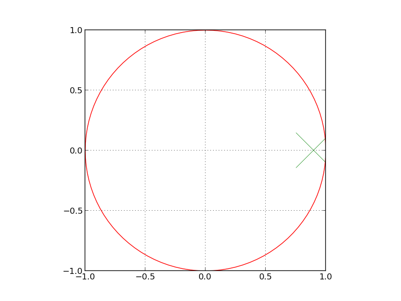
![y[n] = x[n] + 0.9y[n-1]](https://s0.wp.com/latex.php?latex=y%5Bn%5D+%3D+x%5Bn%5D+%2B+0.9y%5Bn-1%5D&bg=eeeeee&fg=666666&s=0&c=20201002)
![y[0] = 1](https://s0.wp.com/latex.php?latex=y%5B0%5D+%3D+1&bg=eeeeee&fg=666666&s=0&c=20201002)
![y[1] = .9](https://s0.wp.com/latex.php?latex=y%5B1%5D+%3D+.9&bg=eeeeee&fg=666666&s=0&c=20201002)
![y[2] = .81](https://s0.wp.com/latex.php?latex=y%5B2%5D+%3D+.81&bg=eeeeee&fg=666666&s=0&c=20201002)


![y[n] = x[n] - 2y[n-1]](https://s0.wp.com/latex.php?latex=y%5Bn%5D+%3D+x%5Bn%5D+-+2y%5Bn-1%5D&bg=eeeeee&fg=666666&s=0&c=20201002)
![y[1] = -2](https://s0.wp.com/latex.php?latex=y%5B1%5D+%3D+-2&bg=eeeeee&fg=666666&s=0&c=20201002)
![y[2] = 4](https://s0.wp.com/latex.php?latex=y%5B2%5D+%3D+4&bg=eeeeee&fg=666666&s=0&c=20201002)


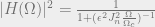
 is the cutoff frequency:
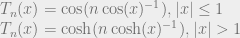
 is the ripple factor, i.e. how much ripple would you allow, and
  is the Chebychev polynomial:

 is the Jacobi elliptic function of n-order. I have no idea how to describe these in a concise way, but they are widely implemented in filter design suites and are tabulated in tons of places, so you don’t have to know the nitty gritty details to implement elliptical filters.
 ![y[n] - .5y[n-1] = x[n]](https://s0.wp.com/latex.php?latex=y%5Bn%5D+-+.5y%5Bn-1%5D+%3D+x%5Bn%5D&bg=eeeeee&fg=666666&s=0&c=20201002)
 ,
, ![y[n] = 1](https://s0.wp.com/latex.php?latex=y%5Bn%5D+%3D+1&bg=eeeeee&fg=666666&s=0&c=20201002) . At the next time step,
. At the next time step, ![y[n] = x[n] + .5y[n-1] = 0 + .5 = .5](https://s0.wp.com/latex.php?latex=y%5Bn%5D+%3D+x%5Bn%5D+%2B+.5y%5Bn-1%5D+%3D+0+%2B+.5+%3D+.5&bg=eeeeee&fg=666666&s=0&c=20201002) . And the next time step,
. And the next time step, ![y[n] = x[n] + .5y[n-1] = 0 + .25 = .25](https://s0.wp.com/latex.php?latex=y%5Bn%5D+%3D+x%5Bn%5D+%2B+.5y%5Bn-1%5D+%3D+0+%2B+.25+%3D+.25&bg=eeeeee&fg=666666&s=0&c=20201002) . And so you can see with every time step, our resulting signal is getting smaller, and it does converge to 0, but it just keeps going and going.
. And so you can see with every time step, our resulting signal is getting smaller, and it does converge to 0, but it just keeps going and going. 
 ,
,
 and SYMMETRIC densities of
  (symmetric meaning
  ) that we are drawing samples from, where g is conditioned on the previous sample we had accepted,
 , which we’ll MIGHT be using to make our decision whether or not to keep or reject the new sample.
 , such that the PDF of the new sample is larger than the previous one, we keep our new sample straight up. Otherwise, we need to do a check against our uniformly distributed value; if our uniformly distributed random sample
  , then we keep the new sample x. Otherwise, we reject x.
 is replaced with the x we just got. Go back to step 1 and keep doing it until we have enough values.
 samples of basically any probability density. The idea behind it is that we can sample a random variable by sampling uniformly underneath the graph of a density function.
  that we are drawing samples from,
 , which we’ll be using to make our decision whether or not to keep or reject the new sample.
 , then we keep x. Otherwise, we reject x.
 so that step 2 actually makes sense, avoiding violating axioms of probability.
  and a cumulative density function
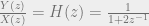
  . We can suggest that random variable Y is a function of X such that
  , meaning the probability of the random variable X being less than or equal to X is equal to Y. Thanks to axioms of probability, we can see that Y is not only distributed only between 0 and 1, but Y has a uniform probability distribution (you can work out the function of a random variable using CDF method and you’ll get things that cancel out and suggest that you have a uniform distribution, regardless of what X is distributed. Something like
 . So we find the inverse of the CDF of X, and just feed it uniform random variables between 0 and 1.
  , and the CDF is
  . We find the inverse of the CDF, so
  . If we plug in uniformly generated numbers, which are generally readily accessible on a computer by some means of pseudorandom number generator, we get exponentially distributed random variables.
  where S is the set of all states we care about, we have a transition matrix that is n x n elements, say a matrix A like the following:
 is the probability of being AT state i, and moving to state j. REMEMBER THIS, because some books like to refer to it the other way around, like i is the target state and j is the previous state, and that changes our notation up entirely here.
 ![X_{0} = [x_{1}, x_{2}, \hdots, x_{n}]](https://s0.wp.com/latex.php?latex=X_%7B0%7D+%3D+%5Bx_%7B1%7D%2C+x_%7B2%7D%2C+%5Chdots%2C+x_%7Bn%7D%5D&bg=eeeeee&fg=666666&s=0&c=20201002) . The subscript of X indicates which time step we’re talking about, and 0 is obvious the start. We can find the probability of being in whatever state at time step t by doing the following
. The subscript of X indicates which time step we’re talking about, and 0 is obvious the start. We can find the probability of being in whatever state at time step t by doing the following so we have a row vector multiplied by our A transition matrix to get us another row vector with the changed probabilities of being at each state at whatever time step. So that’s cool, right? Very handy in terms of calculation. Assuming your transition matrix is legit, like the rows add up to 1 properly, then your X elements should also sum up to 1 all the time. You can prove this but it takes some work, just accept it for now.
  , so when you multiply the row vector Y with the transition matrix, there is no change to the elements of Y, the probabilities remain the same. This stationary distribution typically comes up as a limiting distribution where
  . So yeah, if you want to brute force your way to a stationary distribution, you can calculate it on a computer by doing matrix multiplies over and over until hitting some convergence point.
  , the transpose of the transition matrix, and finding the eigenvector associated with eigenvalue 1, and normalizing it such that it is a legit discrete probability vector. So there’s a clear relation of linear algebra to Markov chains.
 is some radian frequency oscillation rate,
  is obviously time.


 where r is the order of the polynomial and a values are coefficients of the polynomial and an error function defined as
 ![E(x) = W(x)[D(x)-P(x)]](https://s0.wp.com/latex.php?latex=E%28x%29+%3D+W%28x%29%5BD%28x%29-P%28x%29%5D&bg=eeeeee&fg=666666&s=0&c=20201002) where D is the desired “optimal” function of x, and W is how we are weighting the error,
where D is the desired “optimal” function of x, and W is how we are weighting the error,  is a unique polynomial of r order that minimizes
  iff
iff  exhibits AT LEAST
  alternations.
![H(e^{j\omega}) = \sum_{n=0}^{L-1} h[n] \cos(\omega)^{n}](https://s0.wp.com/latex.php?latex=H%28e%5E%7Bj%5Comega%7D%29+%3D+%5Csum_%7Bn%3D0%7D%5E%7BL-1%7D+h%5Bn%5D+%5Ccos%28%5Comega%29%5E%7Bn%7D&bg=eeeeee&fg=666666&s=0&c=20201002) . Then, if we have
. Then, if we have  , then obviously we can see we have a polynomial on our hands. We can define a linear polynomial interpolation problem at extremal points in frequency (for simplicity, let’s set it up Ax=b just like a Vandermonde interp problem) such that
 between
  and
and  between
  .
. of newly designed filter from the constraints we desired at the beginning, and find all of the points in this error function that are
  where
where  is our ripple value. These points are now your new extremal points.